Northwind SQL Analysis : From Raw CSV Files to Advanced SQL

Introduction
The first part of this project focuses entirely on the SQL analysis of the Northwind dataset.
Unlike my previous Superstore project, the objective here was not to immediately build a dashboard or focus primarily on visualization.
Instead, I wanted to understand what happens before the data reaches a visualization tool.
The project therefore starts with raw CSV files and follows the complete process of:
Raw data → SQL Server → Database structure → Relationships → SQL analysis
I also wanted to progressively develop my SQL skills by starting with relatively simple queries and gradually moving towards more advanced concepts.
The progression covered:
- filtering with
WHERE; - pattern matching with
LIKE; - aggregate functions;
GROUP BY;JOIN;- multiple-table
JOINs; LEFT JOIN;- subqueries;
- correlated subqueries;
- nested subqueries;
- CTEs;
- window functions;
LAG().
The objective was not simply to learn individual SQL commands, but to understand how these concepts can be combined to answer increasingly complex questions about the data.
1. Getting the Northwind Dataset
The project started with the Northwind dataset, provided as a collection of CSV files.
The dataset contains several related tables representing customers, orders, products, employees, categories and shippers.
The files I used included:
categories.csvcustomers.csvemployees.csvorder_details.csvorders.csvproducts.csvshippers.csv
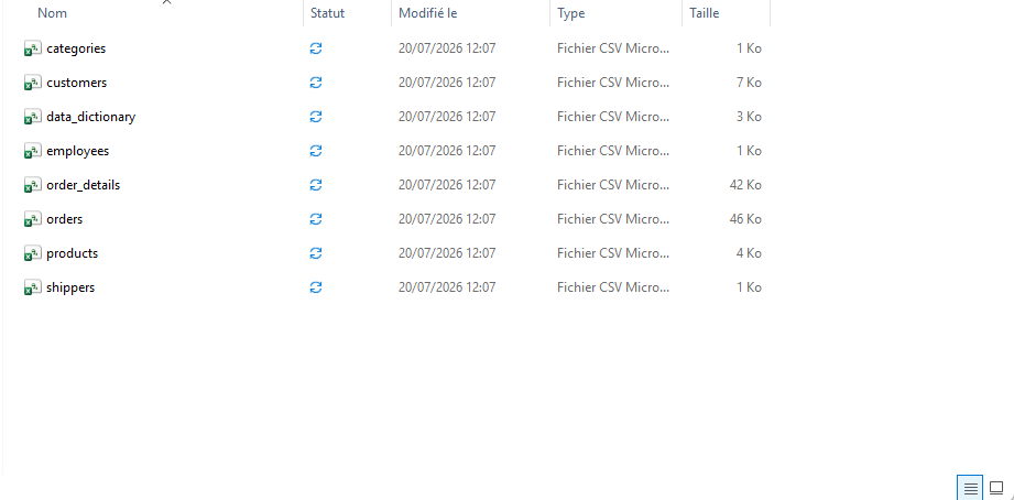
The first step was therefore to get these CSV files ready to be imported into SQL Server.
2. Creating the SQL Server Database
Before importing the CSV files, I created a dedicated database in SQL Server Management Studio (SSMS).
The purpose was to have a structured environment where I could store the Northwind tables and perform the analysis using SQL.

Once the database had been created, I could start working on the individual CSV files.
3. Importing the Northwind Dataset
Once the database had been created, the next step was to bring the Northwind CSV files into SQL Server.
My first approach was to try importing the CSV files directly through the SQL Server interface.
However, I ran into problems with the import process and was not able to use the standard import method successfully.
Rather than continuing to rely on the graphical import interface, I decided to take a more direct SQL approach.
This meant creating the tables myself and then importing the contents of the CSV files using SQL.
3.1 First Attempt Importing the CSV Files
My initial approach was to use the SQL Server import functionality to bring the CSV files directly into the database.
This approach did not work as expected, so I changed the method I was using.
Instead of allowing SQL Server to automatically create the tables from the CSV files, I decided to define the table structure myself.
This also gave me more control over:
- column names;
- data types;
- primary keys;
- foreign keys;
- the structure of each table.
3.2 Creating the Tables Manually
I therefore created the Northwind tables directly in SQL Server before importing the data.
The tables corresponded to the different CSV files:
| CSV file | SQL table |
|---|---|
categories.csv | Categories |
customers.csv | Customers |
employees.csv | Employees |
order_details.csv | Order_Details |
orders.csv | Orders |
products.csv | Products |
shippers.csv | Shippers |
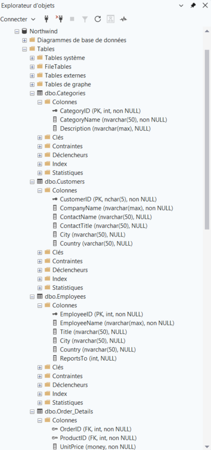
Creating the tables first meant that I could define the database structure myself rather than relying on SQL Server to infer everything from the CSV files.
This became particularly important when I later defined the primary and foreign keys.
3.3 Importing the CSV Files Using BULK INSERT
Once the tables had been created, I needed to populate them with the data contained in the CSV files.
For this, I used SQL Server’s BULK INSERT statement.
Instead of importing the files through a graphical wizard, I instructed SQL Server directly to read the CSV files and insert their contents into the corresponding tables.
The general process was:
CSV file → BULK INSERT → SQL table
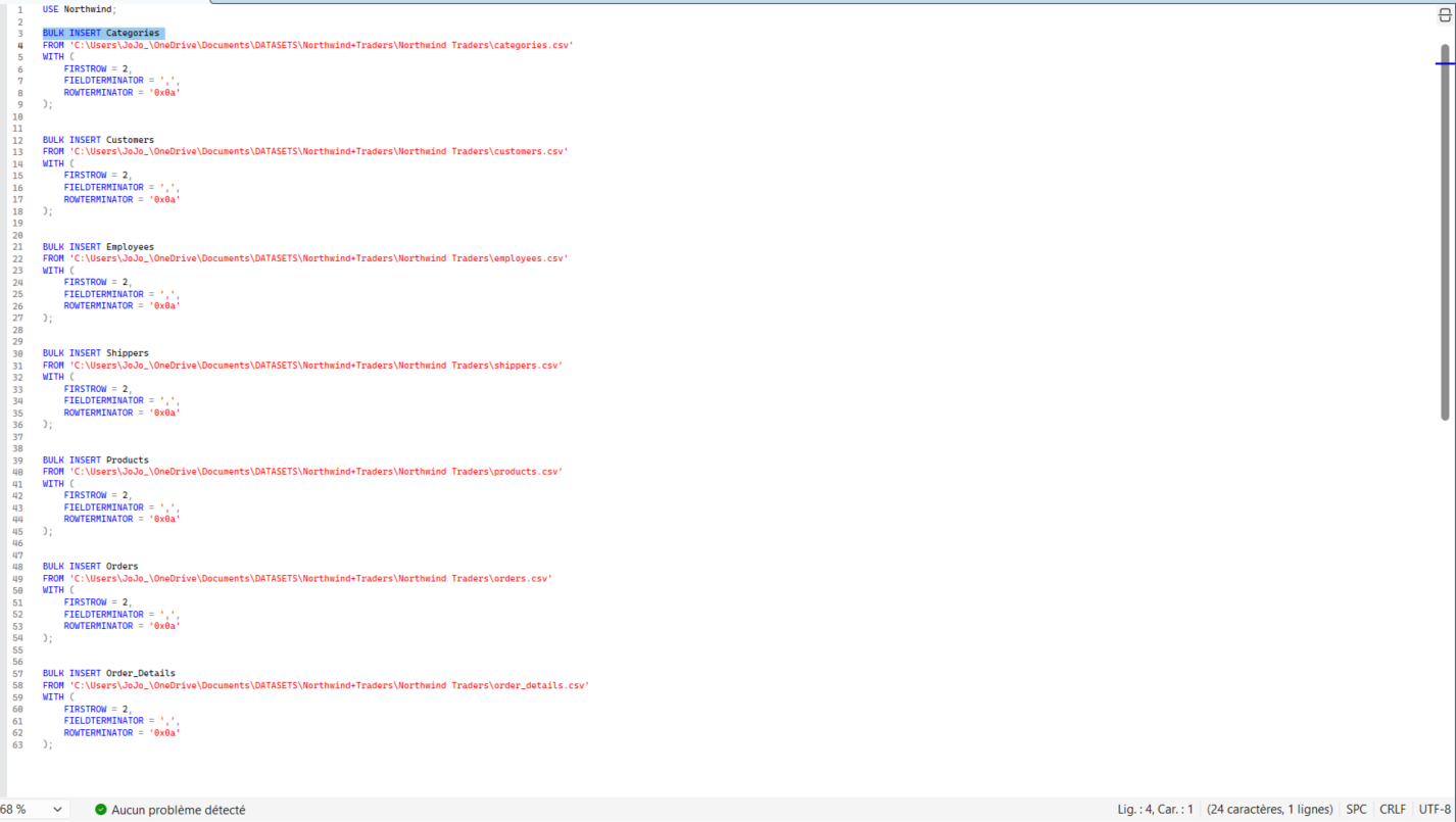
I repeated the same process for the other Northwind tables.
The process therefore became:
Create table
Specify the table structure
Use BULK INSERT
Load the CSV data
Verify the imported records
This approach gave me a better understanding of what was actually happening during data import instead of relying entirely on a graphical interface.
3.4 Verifying the Imported Data
After loading each CSV file, I checked that the data had actually been inserted into the corresponding table.
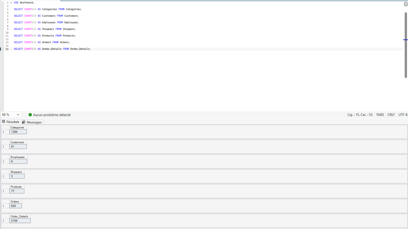
I also checked the tables inside SQL Server Management Studio.
At this point, the CSV files had successfully been transformed into a structured relational database.
The database was now ready for the next stage:
defining the relationships between the tables.
4. Understanding the Database Structure
Before starting the SQL analysis, I needed to understand how the different tables were connected.
Northwind is a relational database, meaning that information is distributed across multiple tables and connected through keys.
For example:
Customers → Orders
The CustomerID stored in the Orders table allows an order to be associated with a customer.
Another relationship is:
Orders → Order_Details
The OrderID connects an order to its individual order details.
And:
Products → Order_Details
The ProductID connects an individual order detail to the product that was purchased.
A simplified representation is therefore:
Customers → Orders → Order_Details → Products
Other tables such as Employees, Shippers and Categories are connected through their respective keys.
5. Defining Primary Keys
Once the tables had been created and populated, I identified the columns that uniquely identify records within each table.
Examples include:
Customers→CustomerIDOrders→OrderIDProducts→ProductIDEmployees→EmployeeIDCategories→CategoryIDShippers→ShipperID
These columns were defined as Primary Keys.
A primary key uniquely identifies a record inside a table.
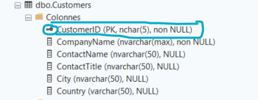
A good example would be the Customers table with CustomerID identified as the primary key.
6. Defining Foreign Keys and Relationships
After defining the primary keys, I created the relationships between the tables using foreign keys.
For example:
Customers.CustomerID → Orders.CustomerID
Here:
Customers.CustomerIDis the primary key.Orders.CustomerIDis the foreign key.
Another relationship is:
Orders.OrderID → Order_Details.OrderID
And another:
Products.ProductID → Order_Details.ProductID
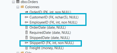
This step was particularly important because these relationships would later be used when writing JOIN queries.
7. Starting the SQL Analysis
Once the database had been imported, structured and connected, I could finally begin analysing the data.
I deliberately started with very simple queries.
The objective was to build my understanding progressively rather than immediately jumping into complicated analytical queries.
The progression was:
SELECT → WHERE → ORDER BY → Aggregations → GROUP BY → JOINs → Subqueries → CTEs → Window Functions
The following sections show selected examples from that progression.
8. Basic Data Retrieval — SELECT
The first concept I worked with was SELECT.
The purpose was simply to retrieve information from a table.
For example, I retrieved customer contact names from the Customers table.
At this stage, I was learning the basic structure of a SQL query:
SELECT → FROM → Table
The query was simple, but it established the foundation for everything that followed.
9. Filtering Data with WHERE
Once I understood how to retrieve data, I moved on to filtering.
The next question was more specific:
Which products have a unit price between 20 and 50?
This introduced:
WHERE;- comparison operators;
AND;ORDER BY.

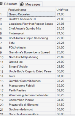
This represented an important progression because SQL was no longer simply retrieving all records.
I was now asking SQL to return only records matching specific conditions.
10. Aggregate Functions
After learning how to retrieve and filter individual records, I started looking at the data from a more analytical perspective.
I worked with aggregate functions such as:
COUNT();SUM();AVG();MIN();MAX().
For example, I calculated the most expensive and cheapest products.
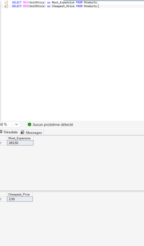
This represented an important change in the type of analysis.
Instead of returning individual records, SQL was now calculating a metric from the dataset.
11. GROUP BY
The next step was to group information.
Instead of asking how many customers existed in total, I wanted to know how many customers existed in each country.
This introduced the GROUP BY clause.
This allowed me to compare different groups within the dataset rather than looking at the dataset as a whole.
12. JOIN : Connecting Tables
At this point, I had mainly been working with individual tables.
However, one of the main advantages of a relational database is the ability to combine information from multiple tables.
This is where JOIN became essential.
For example, an order contains a CustomerID, while the customer’s name is stored in the Customers table.
I therefore needed to connect the two tables.
The JOIN uses the matching key between the two tables.
This was the point where the relationships created during the database setup became directly useful for analysis.
13. Multiple JOINs
After understanding a basic JOIN, I increased the complexity by joining several tables together.
The objective was to retrieve information about:
- the order;
- the customer;
- the employee;
- the shipper.
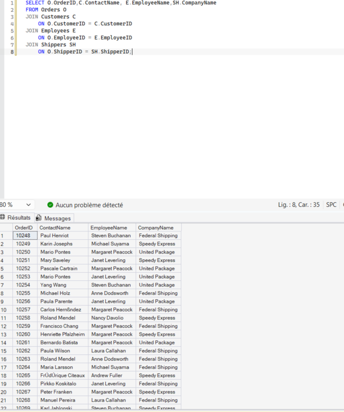
This demonstrated how several relationships within the database could be combined to create a richer result.
14. JOIN + WHERE : Answering a Business Question
I then combined the concepts I had learned so far.
The question became:
Which products have been purchased by customers from Germany?
To answer this, I needed to connect:
Customers → Orders → Order_Details → Products
This represented an important change in the way I was using SQL.
I was no longer writing queries only to practise SQL syntax.
I was beginning to use SQL to answer actual business questions.
15. Calculating Revenue
The next stage was to create an actual business metric.
Using the order details, I calculated revenue using:
Unit Price × Quantity × (1 − Discount)
I then used this calculation to identify the categories generating the highest revenue.
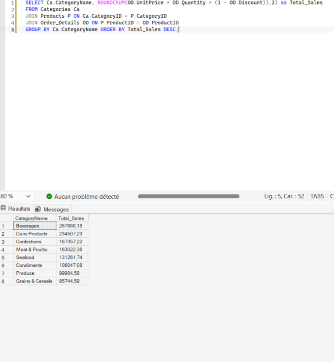
This query combined several concepts that I had previously learned individually:
JOIN;SUM();- calculations;
GROUP BY;ORDER BY.
The question had now evolved from:
What data is in the database?
to:
Which categories generate the most revenue?
16. LEFT JOIN : Finding Missing Relationships
I then used JOINs for another type of problem.
Instead of looking for records that matched between tables, I wanted to identify customers who had never placed an order.
This introduced the combination of:
LEFT JOIN + IS NULL
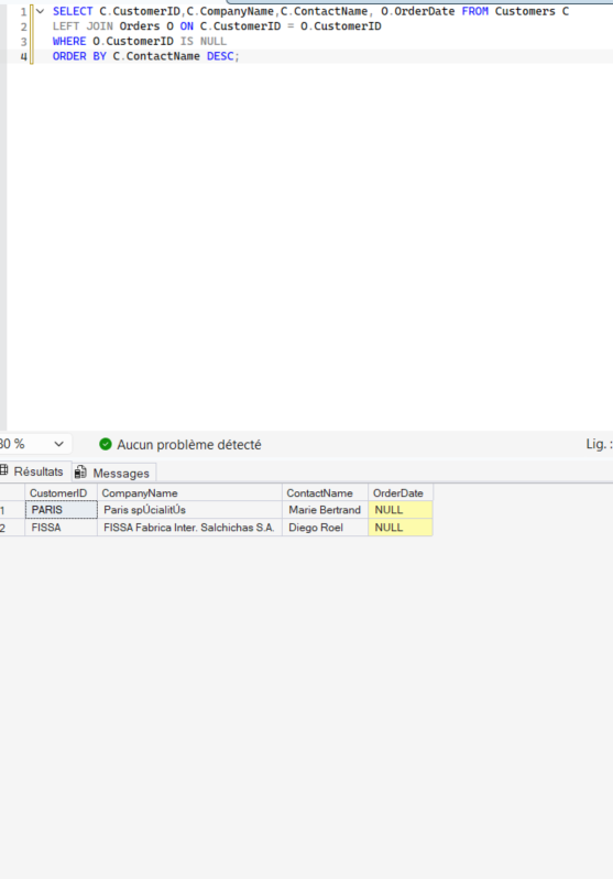
This demonstrated that JOINs can also be used to identify missing relationships between tables.
17. Subqueries : Comparing Against an Average
After becoming comfortable with joins and aggregations, I moved towards more advanced SQL logic.
The question was:
Which products are more expensive than the average product price?
This required a query inside another query.
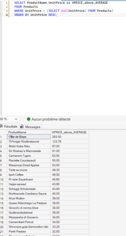
The inner query calculates the average product price.
The outer query then compares each product against that value.
The logic is:
Calculate average → Compare products → Keep products above average
This was an important step because SQL was now being used to produce one result and then use that result as part of another calculation.
18. Correlated Subqueries
I then increased the complexity further.
Instead of comparing every product against the average price of all products, I wanted to compare each product against the average price of products within its own category.
This required a correlated subquery.
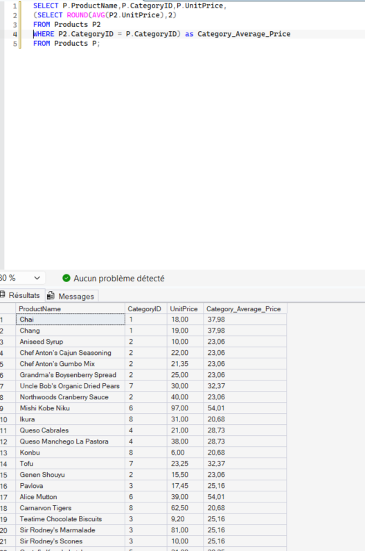
The important difference is that the inner query refers back to the current row of the outer query.
This meant that the average was calculated according to the product’s category.
The progression was now:
Basic query → Aggregate → Subquery → Correlated subquery
19. Common Table Expressions (CTEs)
As the analytical questions became more complicated, I needed a way to structure my queries into clearer steps.
This led me to Common Table Expressions, commonly called CTEs.
I first used a CTE to calculate monthly sales.
A CTE allowed me to create an intermediate result that could then be used by the main query.
The logical structure became:
Orders + Order_Details → Monthly Sales → Further Analysis
This made more complex queries easier to organise.
20. CTE + Window: Function Cumulative Sales
Once I understood CTEs, I combined them with a window function.
The objective was to calculate cumulative sales over time.
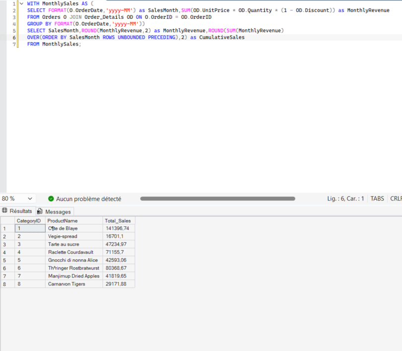
The result allowed me to compare:
- the revenue generated during each individual month;
- the revenue accumulated up to that month.
This was another major progression because I was now analysing values across rows while preserving the individual monthly records.
21. Final SQL Analysis: Month-over-Month Growth
For the final stage of this SQL analysis, I wanted to calculate how sales changed compared with the previous month.
The question was:
How much did sales increase or decrease compared with the previous month?
To answer this, I used:
- CTEs;
- aggregation;
LAG();- calculated columns;
- percentage calculations.
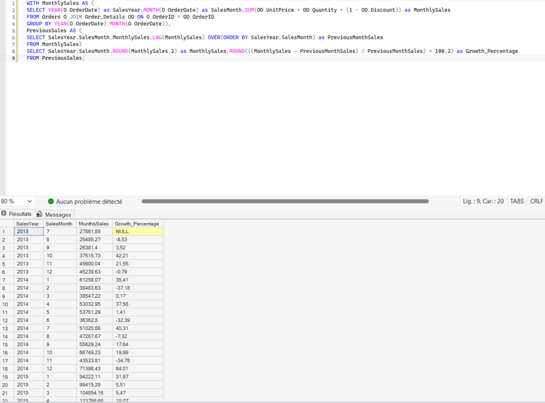
The logic can be simplified as:
Calculate monthly sales
Retrieve previous month’s sales
Compare current month against previous month
Calculate percentage growth
The LAG() function allowed me to access the previous month’s value while keeping the current month’s row.
This represented the most advanced SQL analysis of this first part of the project.
22. The Progression of My SQL Learning
Looking back at the project, the queries were not isolated exercises.
They formed a progression in my understanding of SQL.
The development can be summarised as:
Database creation
CSV import using BULK INSERT
Primary and foreign keys
Relationships
SELECT
WHERE
ORDER BY
Aggregate functions
GROUP BY
JOIN
Multiple JOINs
Business calculations
LEFT JOIN
Subqueries
Correlated subqueries
CTEs
Window functions
LAG()
Month-over-month analysis
The important progression was therefore not simply learning more SQL commands.
It was learning how to combine these concepts to answer increasingly complex questions.
I started with:
How do I retrieve information?
Then:
How do I filter and summarise information?
Then:
How do I combine information from different tables?
And finally:
How can I use SQL to perform actual business analysis?
Conclusion
This first part of the Northwind project allowed me to work through the SQL analysis process from the database setup to advanced analytical queries.
I started with the raw CSV files.
My initial attempt was to import them directly through SQL Server, but after encountering problems with that approach, I changed my method.
Instead, I created the tables myself and used BULK INSERT to load the CSV data into SQL Server.
This gave me a better understanding of the database structure and allowed me to control the tables before establishing their relationships.
I then identified the primary keys, defined the foreign keys and created the relationships between the different tables.
From there, I progressively developed my SQL analysis.
The progression took me from:
Basic data retrieval
to:
Filtering and aggregation
then:
Grouping and JOINs
then:
Business calculations
and finally:
Subqueries, CTEs and window functions
The final month-over-month analysis represents the most advanced SQL stage of this project.
More importantly, I was no longer simply practising SQL syntax.
I was using SQL to answer questions about customers, products, orders, revenue and sales performance.
This established the analytical foundation for the second part of the project.
Part 2: Connecting SQL Server to Power BI
The next stage of the project will move away from SQL syntax and towards visualization.
Now that the database has been structured and analysed using SQL Server, I can use it as the foundation for a Power BI project.
The next part will focus on:
- Connecting Power BI to SQL Server;
- importing the required tables;
- checking the existing relationships;
- preparing the data model;
- creating DAX measures;
- building visualizations;
- analysing the results;
- creating the final interactive dashboard.
The question will therefore change from:
How can I analyse the data using SQL?
to:
How can I transform this analysis into an interactive Power BI report?
Project Progression
This project will therefore be divided into two major stages.
Part 1: SQL Analysis
Raw CSV files
SQL Server database
Manual table creation
BULK INSERT
Primary and foreign keys
Relationships
Basic SQL
JOINs
Subqueries
CTEs
Window Functions
Advanced SQL analysis
Part 2: Power BI Analysis
SQL Server
Power BI connection
Data model
DAX
Visualisations
Dashboard
The objective is to show the complete journey from raw relational data to a finished analytical report.
Thank you for taking the time to explore this project. It forms part of my data analytics portfolio and showcases my ability to build a relational database from scratch and write SQL ranging from basic filtering to advanced analytical queries using joins, subqueries, CTEs, and window functions. Feedback and suggestions are always welcome.